3  Environmental data

3.1 Land Cover and Land Use

Land coverage and use was touched in Section 2.3, where the focus was mainly on OpenStreetMap data as a source. However there is more datasets available, based on satellite observations.

3.1.1 ESA WorldCover

European Space Agency (ESA) released a freely accessible global land coverage data sets. These data sets are based on Sentinel-1 and Sentinel-2 data and contains 11 land cover classes with overall accuracy over 75%. The first set was released in 2021, the second, with higher quality, in 2022 (Zanaga et al. 2021, 2022). The data is accessible through AWS Open Data Registry, Zenodo and/or Terrascope. Terrascope provides the data as WM(T)S services as well, which can be used directly in QGIS:

  • WMTS: https://services.terrascope.be/wmts/v2
  • WMS: https://services.terrascope.be/wms/v2
Code
worldcover_file <- "data/WorldCover_PUM_V2.0.pdf"
if(!file.exists(worldcover_file)) {
  worldcover_file <- "https://esa-worldcover.s3.eu-central-1.amazonaws.com/v200/2021/docs/WorldCover_PUM_V2.0.pdf"  
}

esa_worldcover_maps_data <- "data/esa_worldcover.rds"
if(!file.exists(esa_worldcover_maps_data)) {
  t <- tabulizer::extract_tables(file = worldcover_file,
                                 pages = 15,
                                 method = "stream",
                                 output = "data.frame")[[1]]
  
  colnames(t) <- c("map_code", "land_cover_class", "lccs_code", "definition", "color_code_rgb")
  t <- t[2:nrow(t),]
  t$map_code <- as.numeric(t$map_code)
  
  map_codes <- t$map_code[!is.na(t$map_code)]
  
  merge_cels <- function(column = "", start = 10) {
    stop <- map_codes[which(map_codes == start)+1]
    a <- which(t$map_code == start)
    if(is.na(stop)) {
      b <- nrow(t)
    } else {
      b <- which(t$map_code == stop)-1
    }
    t[a:b, column] |>
      paste(collapse = " ") |>
      stringr::str_trim()
  }
  
  n <- t[1:11,] 
  
  n$map_code <- map_codes
  
  n <- n |>
    dplyr::rowwise() |>
    dplyr::mutate(land_cover_class = merge_cels(column = "land_cover_class", start = map_code),
                  lccs_code = merge_cels(column = "lccs_code", start = map_code),
                  definition = merge_cels(column = "definition", start = map_code),
                  color_code_rgb = merge_cels(column = "color_code_rgb", start = map_code),
                  color = rgb(red = strsplit(color_code_rgb[[1]], split = "[,]")[[1]][1],
                              green = strsplit(color_code_rgb[[1]], split = "[,]")[[1]][2],
                              blue = strsplit(color_code_rgb[[1]], split = "[,]")[[1]][3],
                              maxColorValue = 255)
    )
  saveRDS(n, file = "data/esa_worldcover.rds")
} else {
  n <- readRDS(file = "data/esa_worldcover.rds")
}

n[,1:5] |>
  kableExtra::kable(escape = FALSE,
                    col.names = c("Map code", "Land cover class",
                                  "LCCS code", "Definition", "Color code (RGB)")) |>
  kableExtra::kable_classic_2() |>
  kableExtra::column_spec(5, background = n$color, width = "12%")
Table 3.1: ESA WorldCover classes definition and color codes for layers (Van De Kerchove 2022)
Map code Land cover class LCCS code Definition Color code (RGB)
10 Tree cover A12A3 // A11A1 A24A3C1(C2)- R1(R2) This class includes any geographic area dominated by trees with a cover of 10% or more. Other land cover classes (shrubs and/or herbs in the understorey, built-up, permanent water bodies, ...) can be present below the canopy, even with a density higher than trees. Areas planted with trees for afforestation purposes and plantations (e.g. oil palm, olive trees) are included in this class. This class also includes tree covered areas seasonally or permanently flooded with fresh water except for mangroves. 0,100,0
20 Shrubland A12A4 // A11A2 This class includes any geographic area dominated by natural shrubs having a cover of 10% or more. Shrubs are defined as woody perennial plants with persistent and woody stems and without any defined main stem being less than 5 m tall. Trees can be present in scattered form if their cover is less than 10%. Herbaceous plants can also be present at any density. The shrub foliage can be either evergreen or deciduous. 255, 187, 34
30 Grassland A12A2 This class includes any geographic area dominated by natural herbaceous plants (Plants without persistent stem or shoots above ground and lacking definite firm structure): (grasslands, prairies, steppes, savannahs, pastures) with a cover of 10% or more, irrespective of different human and/or animal activities, such as: grazing, selective fire management etc. Woody plants (trees and/or shrubs) can be present assuming their cover is less than 10%. It may also contain uncultivated cropland areas (without harvest/ bare soil period) in the reference year 255, 255, 76
40 Cropland A11A3(A4)(A5) // A23 Land covered with annual cropland that is sowed/planted and harvestable at least once within the 12 months after the sowing/planting date. The annual cropland produces an herbaceous cover and is sometimes combined with some tree or woody vegetation. Note that perennial woody crops will be classified as the appropriate tree cover or shrub land cover type. Greenhouses are considered as built-up. 240, 150, 255
50 Built-up B15A1 Land covered by buildings, roads and other man-made structures such as railroads. Buildings include both residential and industrial building. Urban green (parks, sport facilities) is not included in this class. Waste dump deposits and extraction sites are considered as bare. 250, 0, 0
60 Bare / sparse vegetation B16A1(A2) // B15A2 Lands with exposed soil, sand, or rocks and never has more than 10 % vegetated cover during any time of the year 180, 180, 180
70 Snow and Ice B28A2(A3) This class includes any geographic area covered by snow or glaciers persistently 240, 240, 240
80 Permanent water bodies B28A1(B1) // B27A1(B1) This class includes any geographic area covered for most of the year (more than 9 months) by water bodies: lakes, reservoirs, and rivers. Can be either fresh or salt-water bodies. In some cases the water can be frozen for part of the year (less than 9 months). 0, 100, 200
90 Herbaceous wetland A24A2 Land dominated by natural herbaceous vegetation (cover of 10% or more) that is permanently or regularly flooded by fresh, brackish or salt water. It excludes unvegetated sediment (see 60), swamp forests (classified as tree cover) and mangroves see 95) 0, 150, 160
95 Mangroves A24A3C5-R3 Taxonomically diverse, salt-tolerant tree and other plant species which thrive in intertidal zones of sheltered tropical shores, overwash islands, and estuaries. 0, 207, 117
100 Moss and lichen A12A7 Land covered with lichens and/or mosses. Lichens are composite organisms formed from the symbiotic association of fungi and algae. Mosses contain photo-autotrophic land plants without true leaves, stems, roots but with leaf-and stemlike organs. 250, 230, 160

The data can be accessed from AWS using aws cli. To list the content of the storage you can use:

aws s3 ls --no-sign-request s3://esa-worldcover/

and to sync it with local filesystem:

aws s3 sync --no-sign-request s3://esa-worldcover/v200/2021/map /local/path

The other option would be to mount it as a local file system using s3fs:

s3fs esa-worldcover /local/path -o public_bucket=1

The data is available as TIFF raster tiles in a regular grid (EPSG:4326) with the ellipsoid WGS 1984 (Terrestrial radius=6378 km). The resolution of the grid is 1/12000\(\deg\) corresponding to ~ 10 m at equator. The individual tile cover 3x3 degrees of longitude/latitude, and the filenames are in form:

ESA_WorldCover_10m_2021_v200_N06E012_Map.tif

where NxxExxx (or SxxWxxx) corresponds to latitude (Nort or South) and longitude (West or East). The single file can be downloaded with:

aws s3 cp --no-sign-request s3://esa-worldcover/v200/2021/map/ESA_WorldCover_10m_2021_v200_N51E015_Map.tif /local/file.tif

or from URL:

https://esa-worldcover.s3.eu-central-1.amazonaws.com/v200/2021/map/ESA_WorldCover_10m_2021_v200_N51E015_Map.tif

The AWS buckets can be accessed with {aws.s3} package (Leeper 2024) however rasters can be accessed directly by rast() function from {terra} package (Hijmans 2024) thanks to underlying GDAL Virtual File Systems. First of all we can download FlatGeobuf file containing a layer with tile names and their corresponding polygons:

esa_tiles <- sf::st_read("https://esa-worldcover.s3.eu-central-1.amazonaws.com/esa_worldcover_grid.fgb")
Simple feature collection with 6 features and 1 field
Geometry type: POLYGON
Dimension:     XY
Bounding box:  xmin: 144 ymin: -57 xmax: 171 ymax: -42
Geodetic CRS:  WGS 84
  ll_tile                       geometry
1 S54E168 POLYGON ((168 -54, 168 -51,...
2 S54E165 POLYGON ((165 -54, 165 -51,...
3 S57E159 POLYGON ((159 -57, 159 -54,...
4 S57E156 POLYGON ((156 -57, 156 -54,...
5 S45E144 POLYGON ((144 -45, 144 -42,...
6 S45E147 POLYGON ((147 -45, 147 -42,...
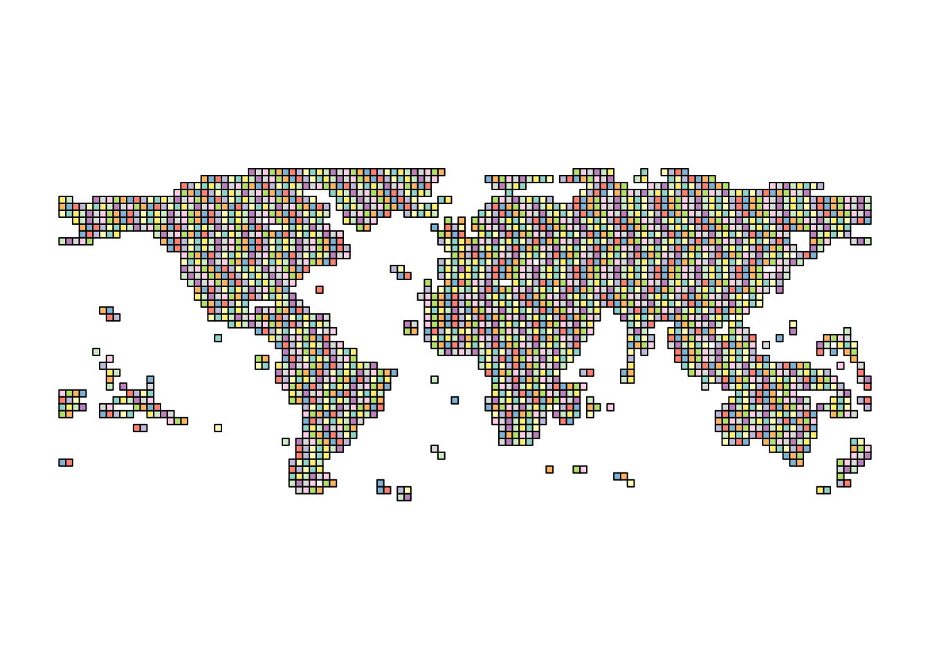
Figure 3.1: Spatial coverage of WorlCover data

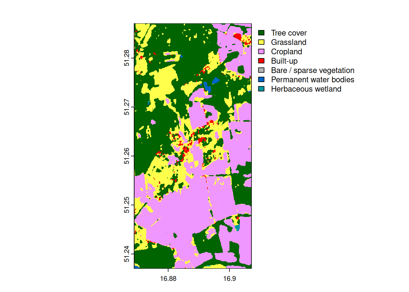
Having tile names (column ll_tile in esa_tiles sf data frame) we can easy find a requested tile(s) by filtering the data frame by our area of interest. Below an example for land cover classes for my village and surroundings. The first step is to find bounding box of the village (getbb() from {osmdata}):

l <- osmdata::getbb("Lubnów, trzebnicki", format_out = "sf_polygon")

The next step is to subset our esa_tiles data frame by l to find the tile(s) which intersects with. It can be done by simple subseting:

b <- esa_tiles[l, ,]
tile_name <- b[[1, "ll_tile"]]
tile_name
[1] "N51E015"

or by st_filter() function

tile_name <- esa_tiles |>
  sf::st_filter(l) |>
  sf::st_drop_geometry() |>
  as.character()
tile_name
[1] "N51E015"

In next step we have to get the proper raster, crop it to the village bounding box, (re)assign levels and table colors. Please note, the levels and colors corresponds to land cover classes and colors from Table 3.1.

terra::setGDALconfig("AWS_NO_SIGN_REQUEST=YES")
url <- paste0("s3://esa-worldcover/v200/2021/map/ESA_WorldCover_10m_2021_v200_", tile_name, "_Map.tif")
r <- terra::rast(url)

w <- terra::crop(r, terra::vect(l)) 

levels(w) <- n[c("map_code", "land_cover_class")] |>
  as.data.frame()
terra::coltab(w) <- n[c("map_code", "color")] |>
  as.data.frame()

terra::plot(w)

It’s worth to mention that {geodata} package have landcover() function, which can download downsampled to 30-seconds per pixel rasters for specific land coverage class.

geodata::landcover(var = "moss", path = tempdir())

3.2 Climate

Key climatic variables are:

  • temperature (°C) (minimum, maximum, average, above ground or at 2 m height)
  • precipitation (mm),
  • solar radiation (kJ m-2 day-1),
  • wind speed (m s-1),
  • water vapor (cm liquid water) and water vapor pressure (kPa),
  • probability of occurrence of snow, snow thickness (cm),
  • soil moisture (cm liquid water),

Those data can be provided as point data sets (per station) or as gridded data sets obtained from analysis or modeling of the past and current climate data.

3.2.1 Stations data

Integrated Surface Database

The Integrated Surface Database (ISD) (Smith, Lott, and Vose 2011; Del Greco et al. 2006; Lott 2004) is a global database that consists of hourly surface observations compiled from numerous sources into a single common ASCII format and common data model. It integrated data from numerous data sources and provides many parameters like temperature and dew point, wind speed and direction, precipitation etc. Data can be accessed from ncei.noaa.gov portal or directly from server where the data is divided by year, and for every station a gziped text file is provided. Data format, described in “Federal Climate Complex Data Documentation for Integrated Surface Data (ISD)” (2018), covers among others: date and time of observation, longitude, latitude and elevation of station, wind direction and speed, sky conditions, visibility distance, air temperature and dev point temperature, atmospheric pressure, precipitation and snow depth. Stations, coded like 040180-16201 can be translated to station names and their physical locations using isd-history.csv file.

Code
isd_stations <- read.csv("https://www.ncei.noaa.gov/pub/data/noaa/isd-history.csv")

isd_stations |>
  dplyr::slice_sample(n = 10) |>
  kableExtra::kable() |>
  kableExtra::kable_classic_2()
Table 3.2: A sample of ISD stations description file which can be used to translate station code to its location
USAF WBAN STATION.NAME CTRY STATE ICAO LAT LON ELEV.M. BEGIN END
949999 315 SCORESBY AS -37.870 145.230 62.0 19561231 19741030
994064 99999 STURGEON POINT LIGHT GLOS WEATHER STATION US MI 44.713 -83.273 184.4 20100325 20240824
136230 99999 SAZAN ISLAND AL 40.500 19.283 240.0 19330516 20240824
727833 4114 CHALLIS (AMOS) US ID KLLJ 44.523 -114.215 1536.2 19990102 20091231
540260 99999 JARUD QI CH 44.567 120.900 266.0 19560820 20240824
027350 99999 VIRRAT AIJANNEVA FI 62.333 23.550 139.5 20090701 20240824
722928 369 MCOLF CAMP PENDLETON RED BEACH AIRPORT US CA KNXF 33.286 -117.456 27.1 20091029 20240722
724463 99999 CHARLES B WHEELER D US MO KMKC 39.117 -94.583 231.0 20000101 20031231
074760 99999 CAUMONT FR LFMV 43.907 4.902 37.8 20040831 20240824
060520 99999 THYBOROEN DA 56.700 8.217 4.0 19730101 20240130

There is a {worldmet} (Carslaw 2023) package which can be used to find the appropriate stations and import the data. Let’s use it to find a stations close to coordinates 15.5°E, 51.5°N and extract the data for one of them:

a <- worldmet::getMeta(lon = 15.5, lat = 51.5)

a[, c(1, 3, 6, 9:11, 15)]
# A tibble: 10 × 7
   usaf   station         call  `elev(m)` begin      end         dist
   <chr>  <chr>           <chr>     <dbl> <date>     <date>     <dbl>
 1 124000 ZIELONA GORA    <NA>      192   1931-01-01 2024-08-24  48.2
 2 124150 LEGNICA         <NA>      124   1937-04-01 2024-08-24  59.0
 3 125000 JELENIA GORA    <NA>      344   1933-06-01 2024-08-24  69.9
 4 123120 BABIMOST        EPZG       59.1 2002-06-03 2024-08-24  74.0
 5 116530 SNEZKA          <NA>     1602   2009-05-01 2024-08-24  86.8
 6 125100 SNIEZKA         <NA>     1613   1952-01-01 2024-08-24  86.8
 7 116030 LIBEREC         <NA>      402.  1937-03-02 2024-08-24  88.2
 8 116430 PEC POD SNEZKOU <NA>      821.  1931-01-01 2024-08-24  90.4
 9 124240 STRACHOWICE     EPWR      123.  1939-01-02 2024-08-24 106. 
10 123100 SLUBICE         <NA>       24   1952-01-02 2024-08-24 113. 

By adding returnMap = TRUE parameter we can see the locations of stations returned:

Let’s download a data for one station and see what’s inside:

station_data <- worldmet::importNOAA(code = "124240-99999",
                     year = 2022,
                     hourly = TRUE,
                     n.cores = 4,
                     path = "data")

station_data |>
  subset(select = c(3, 7:13)) |>
  tail()
# A tibble: 6 × 8
  date                   ws    wd air_temp atmos_pres visibility dew_point    RH
  <dttm>              <dbl> <dbl>    <dbl>      <dbl>      <dbl>     <dbl> <dbl>
1 2022-12-31 18:00:00  5.4   227.     15.5      1016.     23267.     10.0   70.0
2 2022-12-31 19:00:00  5.43  234.     15.2      1016.     23267.      9.33  68.4
3 2022-12-31 20:00:00  6.3   230      15.8      1016.     23267.      9.2   65.0
4 2022-12-31 21:00:00  5.8   227.     15.1      1016.     23267.      9.1   67.7
5 2022-12-31 22:00:00  4.07  224.     14.3      1016.     23267.      8.57  68.7
6 2022-12-31 23:00:00  3.9   220.     14.0      1016.     23267.      8.17  68.0

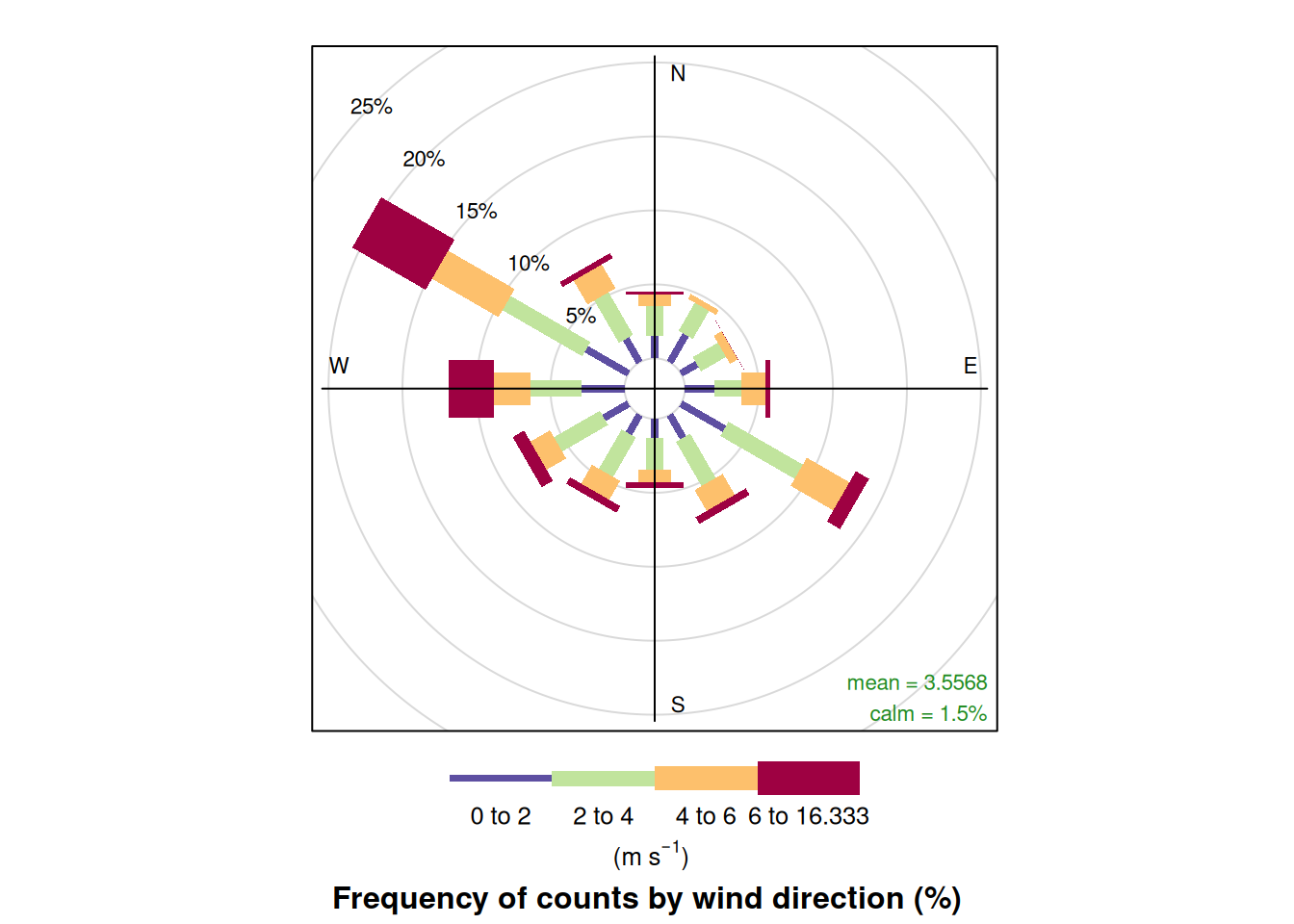
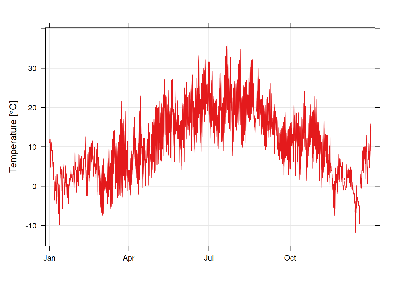
Having data on hand we can perform analysis. A very simple wind rose and temperature diagram for Wrocław-Strachowice station is shown in Figure 3.2.

Code
openair::windRose(station_data)

openair::timePlot(station_data, pollutant = "air_temp",
                  auto.text = FALSE,
                  ylab = "Temperature [\u00B0C]",
                  key = FALSE
                  )
(a)
(b)
Figure 3.2: Examples of station’s data vizualization: direction and wind speed (a) and temperature (b)

Meteorological Aerodrome Report (METAR) data

You may have noticed in Table 3.2, some stations have ICAO (International Civil Aviation Organization) codes. It means, that such hourly data is provided by station located at airport. Copernicus airport at Wrocław-Strachowice is designated with EPWR. The data can be obtained from Aviation Weather Center, historical data is available from ogimet (up to past 20 years) or ASOS Network1. In R we can use {pmetar} package (Cwiek 2023).

library(pmetar)
epwr <- pmetar::metar_get(airport = "EPWR")
epwr
[1] "EPWR 261930Z VRB01KT CAVOK 16/13 Q1023"

From the above report we can read: it was issued on 26 day current month at 19:30 UTC. The wind was blowing from the direction of NA degree and the speed was 1 knots, etc, etc (Milrad 2018).

Code
old <- pmetar::metar_get_historical(airport = "EPWR",
                             start_date = "2022-12-30",
                             end_date = "2022-12-31") |>
  pmetar::metar_decode() 

old |>
  dplyr::mutate(date = as.POSIXct(paste(METAR_Date, " ", Hour, ":00"))) |>
  subset(select = c(date, Wind_speed, Wind_direction, Temperature, Pressure, Dew_point), 
         date >= as.POSIXct("2022-12-31 18:00:00")) |>
  kableExtra::kable() |>
  kableExtra::kable_classic_2()
Table 3.3: Decoded METARs for Wrocław-Strachowice airport
date Wind_speed Wind_direction Temperature Pressure Dew_point
2022-12-31 18:00:00 5.144447 220 16 1016 10
2022-12-31 18:30:00 5.144447 230; variable from 200 to 260 15 1016 10
2022-12-31 19:00:00 4.630002 230; variable from 200 to 260 15 1016 9
2022-12-31 19:30:00 5.658892 230 15 1016 9
2022-12-31 20:00:00 6.173336 230 16 1016 9
2022-12-31 20:30:00 5.658892 230 16 1016 9
2022-12-31 21:00:00 5.658892 230 15 1016 9
2022-12-31 21:30:00 5.658892 220 15 1016 9
2022-12-31 22:00:00 4.630002 230 15 1016 9
2022-12-31 22:30:00 3.601113 210; variable from 180 to 240 14 1016 8
2022-12-31 23:00:00 4.115558 210 14 1016 8
2022-12-31 23:30:00 3.601113 220 14 1016 8

Comparing the data with ISD we can see the METAR reports are issued every 30 minutes.

3.2.2 Gridded data

CHELSA

CHELSA (Climatologies at High resolution for the Earth’s Land Surface Areas) is a data set hosted by the Swiss Federal Institute for Forest, Snow and Landscape Research WSL. The data is based on ERA-Interim climatic reanalysis and contains downscaled to 30 arc sec, ~ 1 km global climate data. (Dirk Nikolaus Karger et al. 2017, 2021). Ver. 2.1 of the data covers monthly datasets of temperatures and precipitation climatologies for years 1979–2019.

Files can be accessed directly from Envicloud server. The filename of each CHELSA data product follows a similar structure including the respective model used, the variable short name, the respective time variables, and the accumulation (or mean) period in the following basic format:

CHELSA_[short_name]_[timeperiod]_[Version].tif

For CMIP6 data:

CHELSA_[short_name]_[timeperiod]_[model] _[ssp] _[Version].tif

Available variable names are listed in Table 3.4. TREELIM model and details (variables: gsl, gsp ... fgd was described by Paulsen and Körner (2014). Köppen-Geiger kg0 and kg1 after Köppen (1936), kg2 classification was updated by Peel, Finlayson, and McMahon (2007), kg3 according to Wissmann (1939), kg4 — new classification by Thornthwaite (1931) and for details of kg5 see (Troll 1964). Miami model for npp variable was described by Lieth (1975).

Table 3.4: Chelsa variable names (Dirk Nikolaus Karger and Zimmermann 2021)
Short name Long name Unit Scale Offset Explanation
bio1 mean annual air temperature °C 0.1 -273.15 Mean annual daily mean air temperatures averaged over 1 year
bio2 mean diurnal air temperature range °C 0.1 0.00 Mean diurnal range of temperatures averaged over 1 year
bio3 isothermality °C 0.1 0.00 Ratio of diurnal variation to annual variation in temperatures
bio4 temperature seasonality °C 0.1 0.00 Standard deviation of the monthly mean temperatures
bio5 mean daily maximum air temperature of the warmest month °C 0.1 -273.15 The highest temperature of any monthly daily mean maximum temperature
bio6 mean daily minimum air temperature of the coldest month °C 0.1 -273.15 The lowest temperature of any monthly daily mean maximum temperature
bio7 annual range of air temperature °C 0.1 0.00 The difference between the Maximum Temperature of Warmest month and the Minimum Temperature of Coldest month
bio8 mean daily mean air temperatures of the wettest quarter °C 0.1 -273.15 The wettest quarter of the year is determined (to the nearest month)
bio9 mean daily mean air temperatures of the driest quarter °C 0.1 -273.15 The driest quarter of the year is determined (to the nearest month)
bio10 mean daily mean air temperatures of the warmest quarter °C 0.1 -273.15 The warmest quarter of the year is determined (to the nearest month)
bio11 mean daily mean air temperatures of the coldest quarter °C 0.1 -273.15 The coldest quarter of the year is determined (to the nearest month)
bio12 annual precipitation amount kg m-2 0.1 0.00 Accumulated precipitation amount over 1 year
bio13 precipitation amount of the wettest month kg m-2 0.1 0.00 The precipitation of the wettest month.
bio14 precipitation amount of the driest month kg m-2 0.1 0.00 The precipitation of the driest month.
bio15 precipitation seasonality kg m-2 0.1 0.00 The Coefficient of Variation is the standard deviation of the monthly precipitation estimates expressed as a percentage of the mean of those estimates (i.e. the annual mean)
bio16 mean monthly precipitation amount of the wettest quarter kg m-2 0.1 0.00 The wettest quarter of the year is determined (to the nearest month)
bio17 mean monthly precipitation amount of the driest quarter kg m-2 0.1 0.00 The driest quarter of the year is determined (to the nearest month)
bio18 mean monthly precipitation amount of the warmest quarter kg m-2 0.1 0.00 The warmest quarter of the year is determined (to the nearest month)
bio19 mean monthly precipitation amount of the coldest quarter kg m-2 0.1 0.00 The coldest quarter of the year is determined (to the nearest month)
gdgfgd0 first growing degree day above 0°c julian day First day of the year above 0°C
gdgfgd5 first growing degree day above 5°c julian day First day of the year above 5°C
gdgfgd10 first growing degree day above 10°c julian day First day of the year above 10°C
fcf frost change frequency count Number of events in which tmin or tmax go above, or below 0°C
gdd0 growing degree days heat sum above 0°c °C 0.1 0.00 Heat sum of all days above the 0°C temperature accumulated over 1 year.
gdd5 growing degree days heat sum above 5°c °C 0.1 0.00 Heat sum of all days above the 5°C temperature accumulated over 1 year.
gdd10 growing degree days heat sum above 10°c °C 0.1 0.00 Heat sum of all days above the 10°C temperature accumulated over 1 year.
gddlgd0 last growing degree day above 0°c julian day Last day of the year above 0°C
gddlgd5 last growing degree day above 5°c julian day Last day of the year above 5°C
gddlgd10 last growing degree day above 10°c julian day Last day of the year above 10°C
gsl growing season length treelim number of days Length of the growing season
gsp accumulated precipiation amount on growing season days treelim kg m-2 0.1 0.00 Precipitation sum accumulated on all days during the growing season based on TREELIM ()
gst mean temperature of the growing season treelim °C 0.1 -273.15 Mean temperature of all growing season days based on TREELIM ()
lgd last day of the growing season treelim julian day Last day of the growing season according to TREELIM ()
fgd first day of the growing season treelim julian day First day of the growing season according to TREELIM ()
ngd0 number of growing degree days number of days Number of days at which tas > 0°C
ngd5 number of growing degree days number of days Number of days at which tas > 5°C
ngd10 number of growing degree days number of days Number of days at which tas > 10°C
kg0 Köppen-Geiger climate classification category Köppen Geiger   Koeppen, W., Geiger, R. (1936): Handbuch der Klimatologie. Gebrüder Borntraeger, Berlin. Wikimedia.
kg1 Köppen-Geiger climate classification category Köppen Geiger without As/Aw differentiation   Koeppen, W., Geiger, R. (1936): Handbuch der Klimatologie. Gebrüder Borntraeger, Berlin. Wikimedia.
kg2 Köppen-Geiger climate classification category Köppen Geiger after Peel et al. 2007   Peel, M. C., Finlayson, B. L., McMahon, T. A. (2007): Updated world map of the Koeppen-Geiger climate classification. Hydrology and earth system sciences discussions, 4(2), 439-473. Free Access.
kg3 Köppen-Geiger climate classification category Wissmann 1939   Wissmann, H. (1939): Die Klima-und Vegetationsgebiete Eurasiens: Begleitworte zu einer Karte der Klimagebiete Eurasiens. Z. Ges. Erdk. Berlin, p.81-92.
kg4 Köppen-Geiger climate classification category Thornthwaite 1931   Thornthwaite, C. W. (1931): The climates of North America: according to a new classification. Geographical review, 21(4), 633-655. JSTOR.
kg5 Köppen-Geiger climate classification category Troll-Pfaffen   Troll, C. & Paffen, K.H. (1964): Karte der Jahreszeitenklimate der Erde. Erdkunde 18, p5-28 Free Access.
scd snow cover days count Number of days with snowcover calculated using the snowpack model implementation in from TREELIM ()
swe snow water equivalent kg m-2 0.1 0.00 Amount of luquid water if snow is melted
npp net primary productivity g C m-2 yr-1 0.1 0.00 Calculated based on the ‘Miami model’, Lieth, H., 1972. “Modelling the primary productivity of the earth. Nature and resources”, UNESCO, VIII, 2:5-10.
pr precipitation amount kg m-2 0.1 0.00 “Amount” means mass per unit area. “Precipitation” in the earth’s atmosphere means precipitation of water in all phases.
tasmax mean daily maximum 2m air temperature °C 0.1 -273.15 Daily maximum air temperatures at 2 metres from hourly ERA5 data
tas mean daily air temperature °C 0.1 -273.15 Daily mean air temperatures at 2 metres from hourly ERA5 data
tasmin mean daily minimum air temperature °C 0.1 -273.15 Daily minimum air temperatures at 2 metres from hourly ERA5 data

Later the data was extended by new variables and got the name BIOCLIM+ (Brun et al. 2022b, 2022a). The variables provides:

  • near-surface relative humidity (hurs)
  • cloud area fraction (clt)
  • near-surface wind speed (sfcWind)
  • vapour pressure deficit (vpd)
  • surface downwelling shortwave radiation (rsds)
  • potential evapotranspiration (pet)
  • climate moisture index (cmi)
  • site water balance (swb)

Detailed description of the variables were provided by Dirk Nikolaus Karger, Brun, and Zimmermann (2022).

And finally, there is a daily sets of data (Dirk N. Karger et al. 2022) which covers the entire globe (except the Arctic Ocean beyond 84°N) at 30 arcsec horizontal and daily temporal resolution from 1979 to 2016. Variables (with short names and units in brackets) included in the CHELSA-W5E5 dataset are: Daily Mean Precipitation (pr) [kg m-2 s-1], Daily Mean Surface Downwelling Shortwave Radiation (rsds) [W m-2], Daily Mean Near-Surface Air Temperature (tas) [K], Daily Maximum Near Surface Air Temperature (tasmax) [K], Daily Minimum Near Surface Air Temperature (tasmin) [K], Surface Altitude (orog) [m], and the CHELSA-W5E5 land-sea mask (mask).

To download CHELSA data in R you can use {ClimDatDownloadR} (Jentsch, Bobrowski, and Weidinger 2024) or {climenv} (Tsakalos et al. 2024) packages.

WorldClim

WorldClim is a database of high spatial resolution global weather and climate data (Fick and Hijmans 2017). It contains monthly data: temperature (minimum, maximum and average), precipitation, solar radiation, vapour pressure and wind speed, aggregated across a target temporal range of 1970–2000. Historical climate data section covers 19 bioclimatic variables BIO1...BIO19. They are average for years 1970–2000. Historical monthly weather data covers monthly weather data for years 1960–2021 downscaled from (Harris et al. 2020). The spatial resolution is 2.5 minutes (~21 km2 at the equator), 5 minutes or 10 minutes. Each zip file contains 120 GeoTiff (.tif) files, for each month of the year (January is 1; December is 12), for a 10 year period. The variables available are average minimum temperature [°C], average maximum temperature [°C] and total precipitation [mm].

To download data in R you can use WorldClim.xxx set of functions in {ClimDatDownloadR} package or worldclim_xxx and cmip6_xxx sets of functions in {geodata} package (Hijmans et al. 2023). There is worldclim() function in {climenv} package as well, it uses geodata::worldclim_tile() function for download.

ERA5 hourly data

ERA5 is the fifth generation ECMWF reanalysis for the global climate and weather for the past 8 decades (Hersbach et al. 2020; Hersbach et al. 2023). Data is available from 1940 onwards with hourly temporal resolution. Horizontal resolution is 0.25 x 0.25° (atmosphere) and 0.5° x 0.5° (ocean waves). You can download it via Copernicus portal. There is a complementary data set named ERA5-Land (Muñoz-Sabater et al. 2021) covering time period from 1981 till today with spatial of 11 km and 1 hour temporal resolutions.

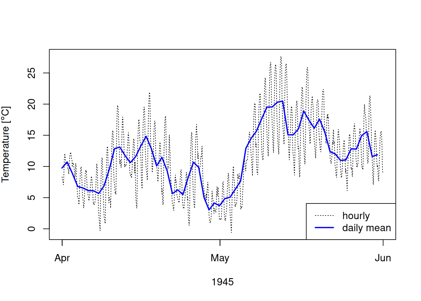
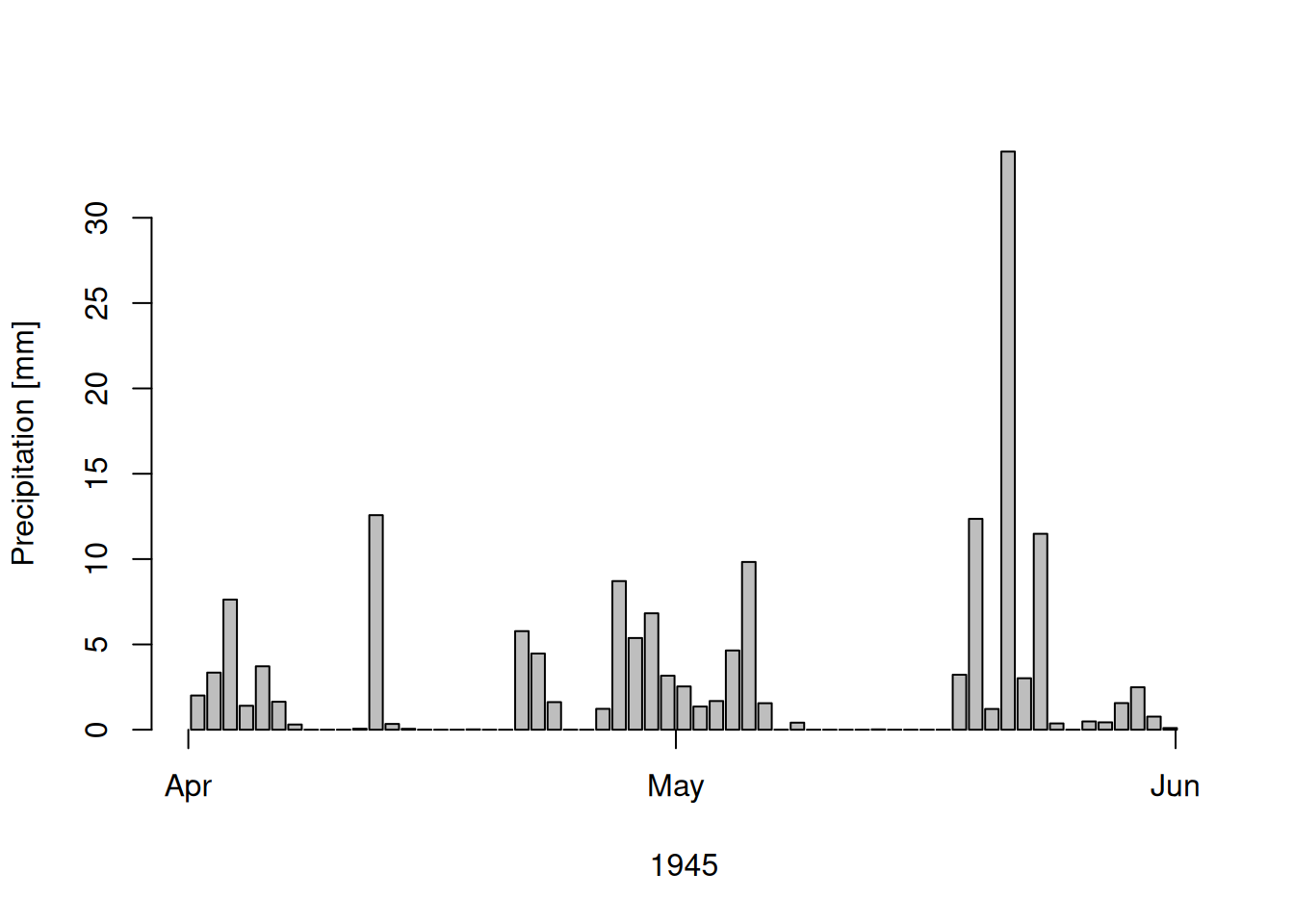
There are few packages which can be used to download the data: {KrigR} (Kusch and Davy 2022) and {ecmwfr} (Hufkens 2023; Hufkens, Stauffer, and Campitelli 2019). In below example, using {ecmwfr}, we are going to check weather conditions in April and May of 1945 in Remagen, Germany.2 After creating ECMWF account and setting up the key in keyring using wf_set_key()3 function we can create data request and download it.

b <- osmdata::getbb("Remagen, Germany")

remagen_lon <- (b[1, 1] + b[1, 2])/2
remagen_lat <- (b[2, 1] + b[2, 2])/2

options(keyring_backend="file")

request <- list(
  product_type = "reanalysis",
  variable = c("2m_temperature", "sea_surface_temperature", "total_precipitation"),
  year = "1945",
  month = c("04", "05"),
  day = c("01", "02", "03", "04", "05", "06", "07", "08", "09", "10", "11", "12", "13", "14", "15", "16", "17", "18", "19", "20", "21", "22", "23", "24", "25", "26", "27", "28", "29", "30", "31"),
  time = c("00:00", "01:00", "02:00", "03:00", "04:00", "05:00", "06:00", "07:00", "08:00", "09:00", "10:00", "11:00", "12:00", "13:00", "14:00", "15:00", "16:00", "17:00", "18:00", "19:00", "20:00", "21:00", "22:00", "23:00"),
  area = c(51, 7, 50, 8),
  format = "netcdf",
  dataset_short_name = "reanalysis-era5-single-levels",
  target = "download.nc"
)

nc <- ecmwfr::wf_request(
  user = "276798",
  time_out = 3600*10,
  request = request,   
  transfer = TRUE,  
  path = "data",
  verbose = TRUE
)

After executing such request you should see a message similar to below one:

Requesting data to the cds service with username 276798
- staging data transfer at url endpoint or request id:
  26df01ad-2c4f-4b70-a568-e58ba43e7deb

- timeout set to 10.0 hours
- polling server for a data transfer
Downloading file
  |============================================================================| 100%
- moved temporary file to -> data/download.nc
- Delete data from queue for url endpoint or request id:
  https://cds.climate.copernicus.eu/api/v2/tasks/26df01ad-2c4f-4b70-a568-e58ba43e7deb

Please note that preparing the data on server side and downloading it might take a long while. Having the data downloaded we can run the analysis.

Code
K <- -273.15

m <- matrix(c(
  remagen_lon, remagen_lat),
  byrow = TRUE, ncol = 2,
  dimnames = list(c("rem"),
                  c("lon", "lat")))

p <- m |>
  terra::vect(m, type = "points", crs = "EPSG:4326")

nc <- "data/download.nc"
r <- terra::sds(nc)

temp2m <- terra::extract(r["t2m"], p, ID = TRUE, bind = TRUE) |>
  as.data.frame()
t_timestamp <- terra::time(r["t2m"])

f <- t(temp2m)
f <- f[3:nrow(f), ]
f <- f + K

f <- f |>
  as.data.frame()
f$t_timestamp <- t_timestamp

daily_means <- f |>
  dplyr::mutate(day = as.Date(t_timestamp)) |>
  dplyr::group_by(day) |>
  dplyr::summarise_at("f", mean) |>
  dplyr::mutate(day = as.POSIXct(paste(day, "00:00:00")))

plot(f$t_timestamp, f$f, type = "l",
     lty = 3,
     xlab = "1945",
     ylab = expression(paste("Temperature [",degree,"C]")),
     )
lines(daily_means$day, daily_means$f, lwd = 2, col = "blue")
legend("bottomright",
       legend = c("hourly", "daily mean"),
       col = c("black", "blue"),
       lty = c(3, 1),
       lwd = c(1, 2)
       )
Figure 3.3: Temperature in Remagen, Germany during April and May 1945
Figure 3.4: Precipitation in Remagen, Germany during April and May 1945

TerraClimate

TerraClimate (Abatzoglou et al. 2018) is a dataset of monthly climate and climatic water balance for global terrestrial surfaces from 1958 to 2023. All data have monthly temporal resolution and a ~4-km (1/24th degree) spatial resolution.

Primary climate variables covers: maximum and minimum temperature, vapor pressure, precipitation accumulation, downward surface shortwave radiation and wind-speed. Derived variables are: reference evapotranspiration (ASCE Penman-Montieth), runoff, actual evapotranspiration, climate water deficit, soil moisture, snow water equivalent, palmer drought severity index and vapor pressure deficit. Detailed description is provided on Climatology Lab. The data is available as netCDF files from THREDDS web server. You can use getTerraClim() function from {climateR} package (Johnson 2024) to access the data in R.

Table 3.5: Abbreviation of the variables used by TerraClimate
Abbreviation Description Units
aet Actual Evapotranspiration, monthly total mm
def Climate Water Deficit, monthly total mm
pet Potential evapotranspiration, monthly total mm
ppt Precipitation, monthly total mm
q Runoff, monthly total mm
soil Soil Moisture, total column - at end of month mm
srad Downward surface shortwave radiation W/m2
swe Snow water equivalent - at end of month mm
tmax Max Temperature, average for month C
tmin Min Temperature, average for month C
vap Vapor pressure, average for month kPa
ws Wind speed, average for month m/s
vpd Vapor Pressure Deficit, average for month kpa
PDSI Palmer Drought Severity Index, at end of month unitless
Note:
Taken from TerraClimate

Global Maps from NASA Earth Observatory and other products

Earth Observatory by NASA provides global monthly images at 10 km spatial resolution and covers years 2000-2024.

Ma, Zhou, Göttsche, Liang, Wang, and Li (2020) created global land surface temperature (LST) dataset, which was generated from NOAA advanced very-high-resolution radiometer (AVHRR) data (1981–2000) and includes three data layers:

The resolution is 0.05° spatially and 1-day temporal. In addition to Zenodo, the data is available at http://glass.umd.edu/LST/ in HDF files.

Based on ERA5 precipitation archive and MODIS monthly cloud cover frequency Dirk Nikolaus Karger, Wilson, et al. (2021) produced global daily 1km land surface precipitation set for the years 2003-2016. In 2021 Zhang et al. (2022) published land surface temperature dataset for 2003-2020 with 1km spatial resolution and on daily (mid-daytime and mid-nightime) basis. The dataset is based on MODIS LST and spatiotemporal gap-filling framework. The data is available for download from Iowa State University in GeoTIFF format. Another approach was taken by Yao et al. (2023) who produced global seamless and high-resolution (30 arcsecond spatial) temperature (with land surface temperature (Ts) and near-surface air temperature (Ta)) dataset for 2001-2020. The data is available at Middle Yangtze River Geoscience Date Center (in Chinese).


  1. The Automated Surface Observing System↩︎

  2. This is a response to Open Data question↩︎

  3. for details please check package documentation↩︎